Mapping Toolbox

MT337 v1.5.0.4

Un logiciel permettant la gestion cartographique de données de caractérisation

UGS : MT337 v1.5.0.4 Catégories: Accessoires, Logiciel

Description

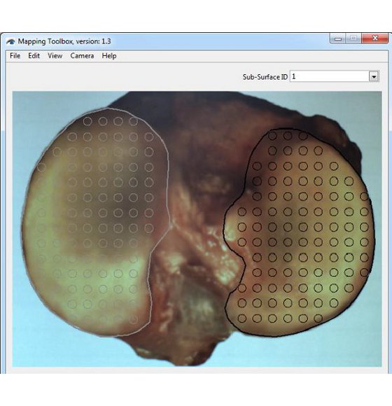
(En anglais seulement) The Mapping Toolbox is a data management software designed to record, manage, analyze and display various types of local characterization perform on the surface of a sample. Characterization data (“.map”, tab-delimited text file) is handled in the form of maps overlaid onto a representative image of the sample surface. Equipped with a camera, the software can also be used as a camera-registration positioning system to capture image of the sample surface and to facilitate manual characterization mapping. This software can manage various type of quantitative value data to create mappings of e.g. stiffness, thickness, chemical content, density, temperature, image path, etc. Eventually, new statistical modules (software add-on) will be released to perform various statistical analyses within a single characterization mapping or among multiple mapping of comparable samples.

Équipé de logiciels intuitifs permettant la collecte efficace des données et des analyse simplifiées
Les données peuvent aussi être analysées dans un logiciel de tierce partie

Documents et ressources (1)

Document

Mapping Toolbox - Manual d'utilisation (English).pdf

Configurations de test (2)

Configuration de test

Cartographie 3D en indentation normale

Configuration de test

Cartographie 3D d'épaisseur

FAQ

Comment créer un gabarit de positions?

(En anglais seulement) In order to facilitate eventual comparison between samples with similar surface, it is recommended to use a boundaries (surface positioning) template to standardize their positioning in the picture frame. This surface positioning template is a “.map” file containing a list of positions outlining the sub-surface’s boundaries and a reference image of the surface of interest.

The reference image should be considered as a representative (average) image of the different samples with a similar surface that will be used for the display of average mapping results taken from multiple comparable surfaces. In order to be representative (average) of all sample surface boundaries within the group of interest, template must be created using enough independent sample surface images. Of course, the number of independent images required will be a function of the extent of boundary variation within the group. Image processing software shall be used to create the representative (average) image.

The boundaries (surface positioning) template can be modified from time to time, in particular when data collection indicates that it is not representative of the population. For this reason, a version number is added to the template which is named using the following convention: “Template-X_SurfaceDescription_vV.map”, where X is the left (L) or right (R) side and V is the version number.

The following is the list of the left and right surface positioning templates currently available:
• Human: Distal Femur, Femoral Condyles, Tibial Plateau, Patella
• Sheep: Femoral Condyles, Tibial Plateau
• Rabbit: Femoral Condyles, Tibial Plateau
• Rat: Femoral Condyles, Tibial Plateau
• Mouse: Femoral Condyles, Tibial Plateau

NOTE. If the sample presents closed sub-surfaces (for example an entire tibial plateau with the medial and lateral plateaus), it is important to describe each of these regions of interest (sub-surfaces) in order to interpolate the mapping within the delimited boundaries.

1. Position the sample in the camera feed or place the camera towards a screen in order to visualize a representative (single or average) image of the sample in the camera feed. Ideally, sample’s surface should be at the center and occupies the maximum space in the image frame while remaining completely visible and allowing some clearance for eventual refraction compensation, if applicable.
2. Create the boundary of the sample surface in the camera feed. Note that it is important to edit/select a sub-surface in the Sub-SurfaceID field before adding a boundary in order to assign the boundary to a sub-surface.
2.1 Choose “Boundary” in “View” of the menu bar to see boundaries in the camera feed.
2.2 Edit the Sub-Surface ID field as defined in the associated protocol.
2.3 Choose “Add Boundary” in “Edit” of the menu bar and click in the camera feed to define the boundary along the sample sub-surface and a closed contour will be created.
2.4 If necessary, choose “Delete Boundary” in “Edit” of the menu bar and click in the camera feed at a boundary point along the sample sub-surface and the closed contour will be reshaped consequently.
2.5 Repeat steps 2.2 to 2.4 for each sub-surface of the sample.

3. Create a blank .map file and name it using the following convention: “Template-X_SurfaceDescription_vV.map”, where X is the left (L) or right (R) side and V is the version number.

Mapping Toolbox – Création de frontière

Commen puis-je dimensionner la vue de dessus de mon échantillon afin d'effectuer une cartographie?

(En anglais seulement) In order to dimension the sample and calibrate its image, two reference marks need to be created on the sample surface as far as possible from each other (ideally not over regions of interest). Marks should be made at approximately the same surface height (ideally at the average horizontal mapping plane, the focal plane of the camera), since it is the top-view image of the sample that is calibrated.

NOTE. Different specified methods can be used to create those reference marks, but they should be made as small as possible (while being clearly visible on the sample and eventually on its image) and should remain mechanically stable and visible after immersion in saline solution (if applicable) and sample manipulation. For example, adding a small drop of India ink over a needle puncture of the cartilage layer at the boundary of the articular surface have proven to lead to good results. It might also be possible to use two distant, clear and unambiguous sample landmarks as reference marks.

1. If already created, open the blank “Filename.map” file to be converted into metric coordinates. Note that the corresponding image “Filename.jpg” should present two visible reference marks. If not already created and if the sample is still in the camera feed, add two reference indicators on the two visible reference marks.
1.1. Choose “Reference 1 (red)” in “Edit” of the menu bar and click in the camera feed at the first reference mark.
1.2. Choose “Reference 2 (blue)” in “Edit” of the menu bar and click in the camera feed at the second reference mark.

2. Set the metric values of the reference marks.
2.1. Choose “Calibration” in “Edit” of the menu bar.
2.2. Report the X and Y metric coordinates of the reference 1 and reference 2 in the “Calibration” pop-up window according to a specific method, currently available is the “Mach-1” method.

“Mach-1” method: This method allows converting the pixels coordinates of the positions into metric coordinates that will be used for a mechanically-controlled surface mapping with the 2 horizontal stages of a multi-axial Mach-1 mechanical tester. The coordinate system used in this method corresponds to the Mach-1 horizontal stages where it is preferable to set X and Y origin at the first reference mark. With the sample/testing chamber mounted onto the Mach-1, move the stages in such a way that the center of the Mach-1’s indenter (its vertical axis) is positioned just over the first reference mark (red indicator), set the position of the X and Y stage to zero position. Repeat the same procedure for the second reference mark (blue indicator), report the X and Y stage position in the “Calibration” pop-up window. Note that since it is possible to increase the effective scanning area (limited by the stages) of the Mach-1 by manually rotating/repositioning the sample or sample/chamber assembly, a configuration index “i” is added to this characterization (by default i=1). Note that it is recommended to keep this configuration index (i) in all Mach-1 raw data generated under configuration (i).

3. Create a “Filename-Dimensioning.map” file, where “Filename” can be defined in an associated protocol.
3.1. Verify that reference 1 and reference 2 indicators are displayed in the camera feed and that their metric coordinates (according to the chosen method) has been reported in the “Calibration” pop-up window.
3.2. Choose “Create .map” in “File” of the menu bar and all positions, boundaries and references displayed in the camera feed will be saved in the .map file and a snapshot image “.jpg” of the camera feed will be saved in the same folder. Also, two characterizations “ScanX(mm)” and “ScanY(mm)” containing the metric coordinates of the two reference marks and those of each position of the grid will be saved.

Mapping Toolbox – La fonctionnalité d’étalonnage

Quelle est la procédure pour créer un gabarit de document ".map"?

(En anglais seulement) NOTE. If no testing chamber is used proceed to step 5.

1. Completely screw the sample holder into the testing chamber and place the sample over it. If applicable, center the sample relative to the holder and rotate it in such a way that its orientation will approximately correspond to that of the corresponding surface positioning template image when seen by the technician in front of the testing chamber. Using a black marker, draw a mark on the top of the sample holder that will be used for the repositioning of the sample over the holder.

2. Remove the sample and unscrew the sample holder.

3. Depending on the sample type, a sample has to be attached to the sample holder following an appropriate method, either with screws and/or cyanoacrylate glue (recommended: Loctite 4013).

“Screws” method: In the case of sample holder (a – see Figure 1a), place the flat sample side in firm contact with the sample holder. Secure it with at least 2 screws from the bottom side. Make sure that the screws remain at least 1 cm away from the surface. In the case of sample holder (b – see Figure 1b), place the flat sample side in firm contact with the sample holder. Secure it from the periphery using its 6cone-ended screws. In the case of sample holder (c – see Figure 1c), place the sample in the middle. Secure it with its 2 screws.

“Glue” method: In the case of any sample holder with a flat portion (see Figure 1), make sure that the bottom surface of the sample and the flat portion of the sample holder are dry to ensure a good adherence. In the case of articular surfaces, apply the glue on the sample bottom (the bony part) and be careful not to touch the cartilage surface. If by mistake the glue touches the sample, try to clean the surface by using a flux of PBS, and report approximately the touched area in the laboratory book. The glued sample should be maintained for at least 1 minute to ensure a good adherence.

4. Screw the assembly into the testing chamber.

5. If required, create two reference points on the surface as per the “Calibration of the sample” section. If required, measure the horizontal distance between the references with a calibrated caliper and report the value (ideally, at a location specified in an associated protocol).

6. Adjust the position of the camera and its focus in such a way that the sample’s surface occupies the maximum space in the live camera feed while remaining completely visible by keeping a margin of about 5% at the 4 sides (right, left, up and down) to accommodate an eventual water refraction compensation, if applicable. It is recommended to use an appropriate surface positioning template to facilitate eventual mapping comparison between samples.
6.1. Choose “Import .map” in “File” of the menu bar.
6.2. Select the corresponding surface positioning template (*.map) and boundaries will be displayed by a closed contour (solid line) in the camera feed.
6.3. Adjust the position of the camera and its focus in such a way that the sample’s surface boundaries fit those of the surface positioning template.

7. Superimpose a position grid to the sample image. Positions could be added one by one according to a snapping grid (aligned) or anywhere on the sample. Also, positions could be imported through a previously created .map file. Note that it is important to edit/select a sub-surface in the Sub-SurfaceID field before adding a position in order to assign the position to a sub-surface.
7.1 If applicable, choose “Import .map” in “File” of the menu bar and select the corresponding position grid and the positions will be displayed by a circled marker in the camera feed.
7.2 If applicable, choose “Grid” in “View” of the menu bar to display a grid of snapping dots in the camera feed.
7.3 Edit the Sub-Surface ID field as defined in the associated protocol.
7.4 Choose “Add Positions” in “Edit” of the menu bar and click in the camera feed to add positions at each location of interest on the sample sub-surface.
7.5 If necessary, choose “Delete Positions” in “Edit” of the menu bar and click in the camera feed at each position that is not overlaid on a location of interest on the sample sub-surface and the position will be deleted from the camera feed.
7.6 Repeat steps 7.3 to 7.5 for each sub-surface of the sample.

8. If required, create the specific boundary of the sample sub-surfaces in order to refine the outline of the mapping surface for this specific sample (using at least 30 boundary points). If needed, surface boundary layer from the positioning template can be deleted first. Note that this step is important for the interpolation of characterization values to the boundary to obtain a complete mapping of the sample surface. Note that it is important to edit/select a sub-surface in the Sub-SurfaceID field before adding a boundary in order to assign the boundary to a sub-surface.
8.1. Choose “Boundary” in “View” of the menu bar to see boundaries in the camera feed.
8.2. Edit the Sub-Surface ID field as defined in the associated protocol.
8.3. Choose “Add Boundary” in “Edit” of the menu bar and click in the camera feed to define the boundary along the sample sub-surface and a closed contour will be created.
8.4. If necessary, choose “Delete Boundary” in “Edit” of the menu bar and click in the camera feed at a boundary point along the sample sub-surface and the closed contour will be reshaped consequently.
8.5. Repeat steps 8.2 to 8.4 for each sub-surface of the sample.

9. If required, add reference indicators on the two reference marks previously created at step 5.
9.1. Choose “Reference 1 (red)” in “Edit” of the menu bar and click in the camera feed at the first reference mark.
9.2. Choose “Reference 2 (blue) in “Edit” of the menu bar and click in the camera feed at the second reference mark.

10. Create this blank “Filename.map” file, where “Filename” is standardized filename format that it is recommended to define in an associated protocol (refer to Appendix I for a recommended file naming convention). When filename standardization is not necessary, any name can be used as “Filename”. Choose “Create .map” in “File” of the menu bar and all positions, boundaries and references displayed in the camera feed will be saved in the .map file and a snapshot image “.jpg” of the camera feed will be saved in the same folder.

Mapping Toolbox – Sample Holders

Comment utiliser la fonction "Clear Position"?

Cliquez sur le panneau d'alimentation de la caméra avec le bouton de droite de votre souris: Cette fonction supprime toutes les positions dans le panneau d'alimentation de la caméra.

Mapping Toolbox – Fenêtre d’alimentation de l’appareil photo

Comment fonctionne la fonction "Sub-SurfaceID"?

Cette fonction permet de sélectionner une sous-surface et d'en éditer le nom (Sub-SurfaceID). Lorsqu'ils sont sélectionnés, les marqueurs de position correspondant à la sous-surface sélectionnée changent de couleur (du gris au noir) dans l'alimentation de la caméra, pour en faciliter la visualisation.

Mapping Toolbox – Sub-SurfaceID

Comment fonctionne la fonction "Template Used"?

(En anglais seulement) This feature indicates which surface positioning template has been used to position the sample in the camera feed. When a surface positioning template is imported into the Mapping Toolbox through the function “Import.map”, this feature indicates the filename (*.map) of the last template imported.

Comment je peux accéder au menu d'aide?

(En anglais seulement) The Help menu contains basic help functionalities (Figure 1) such as the user manual and information about the software/camera firmware.

User Manual - Click on this button to access a PDF file of this User Manual. The Adobe Reader™ must be installed on your computer. Visit https://www.adobe.com for installation details.

À propos - This function provides information about the software, firmware versions and camera serial number (Figure 2)

Mapping Toolbox – Help – About feature

Mapping Toolbox – Help Menu

Comment fonctionne le menu "Camera"?

(En anglais seulement) The Camera menu provides the ability to control the camera feed.

Start - This function starts the camera feed. In this mode, the user can use all features in the Edit menu.
Stop - This function stops the camera feed. In this mode, the user cannot use all features in the Edit menu.

Mapping Toolbox – Menu de l’appareil photo

Comment marche la fonction "Water Refraction (5% Compensation)"?

(En anglais seulement) If required, this function applies a +5% scaling factor to the display of the positions, boundaries and references marks in the camera feed panel (this does not affect the pixel coordinates saved in the .map file). This feature is normally used to compensate for image distortion due to the presence of solution over the sample during manual characterization mapping of a biological sample. Note that the scaling is relative to the center of the grid.

Comment marche la fonction "Set Grid"?

(En anglais seulement) This function will open a pop-up window to allow the user to configure the grid of snapping dots according to either an image-centered square configuration (size, in pixels, can be set from 10 to 200) or table configuration (# columns and # rows can be set from 2 to 50, extended on the full image size).

Mapping Toolbox – La fonctionnalité Définir la grille

Comment puis-je ajouter une frontière à mon échantillon dans les cartographies?

(En anglais seulement) The "Boundary" function displays the boundaries of the surface (or its sub-surface), if defined, to facilitate the positioning of the sample or to see the boundaries when they are created.

"Add Boundary" allows the user to define the boundary of sub-surfaces of the sample. Click the camera feed panel over several points along sample boundary and a closed contour will be created. It is recommended to add boundary points in a clockwise or anti-clockwise order.

Right-click the mouse over the camera feed panel and select "Clear Boundaries" to remove all boundaries in the camera feed panel.

Note. It is important to edit/select a sub-surface in the Sub-SurfaceID field in order to assign a boundary to a sub-surface.

Mapping Toolbox – La fonctionnalité de frontière

Comment marche la fonction "Position ID"?

Cette fonction affiche un numéro de position au bas, à droite de chaque marqueur de position. Ces étiquettes sont des nombres consécutifs commençant par 1 pour la première position ajoutée dans chaque sous-surface.

Mapping Toolbox – La fonctionnalité PositionID

Comment marche la fonction "Grid"?

(En anglais seulement) This function displays a grid of snapping dots, in the camera feed panel, defined by the user. If no values for the grid have been previously defined by the user through the "Set Grid" feature, the software will automatically prompt the user through the "Set Grid" pop-up window. The snapping dots are overlaid on the camera feed panel to make it easier to line up positions added.

Mapping Toolbox – La fonctionnalité Grid

Comment je peux dimensionner mon image de la vue de dessus de mon échantillon pour les cartographies?

(En anglais seulement) This function allows the user to assign the metric coordinates of Reference 1 (red) and Reference 2 (blue). When Mach-1 metric coordinates are entered, ScanX(mm) and ScanY(mm) characterizations are calculated and exported in a ".map" file when created. This function is only applicable when Reference 1 (red) and Reference 2 (blue) markers are displayed in the camera feed panel and when all four fields are different from 0.

Click the camera feed panel on the first reference mark and a red marker will appear. At each click, the red marker will relocate.

Click the camera feed panel on the second reference mark and a blue marker will appear. At each click, the blue marker will relocate.

Right-click the mouse over the camera feed panel and select "Clear References" to remove all references from the camera feed panel.

Mapping Toolbox – La fonctionnalité d’étalonnage

Comment puis-je effacer une position dans une cartographie?

(En anglais seulement) The "Delete Position" function allows the user to delete a position that is not overlaid on a location of interest on the sample. Click the camera feed panel on a position marker to remove it. For faster results, click and hold down the left mouse button on position markers displayed in the camera feed panel and they will be removed on mouse-over until the user releases the left mouse button.

Mapping Toolbox – Edit Menu

Comment marche la fonction "Add Position"?

(En anglais seulement) Note. It is important to edit/select a sub-surface in the Sub-SurfaceID field in order to assign a position to a sub-surface.

This function allows the user to define a position of interest on the sample. Click the camera feed panel at each location of interest and a position marker will be added. When a snapping grid is displayed in the camera feed (grey dots), click and hold down the left mouse button in the camera feed panel and position markers will be added and be aligned to the snapping grid until the user releases the left mouse button.

Future measurements will be taken in the same order that position markers are added to the camera feed panel.

Mapping Toolbox – Edit Menu

Comment marche la fonction "Create .map"?

La fonction "Create .map" crée un fichier ".map" contenant toutes les positions, limites et références affichées dans le panneau d'alimentation de la caméra ainsi qu'une image instantanée ".jpg" de l'alimentation de la caméra.

Mapping Toolbox – File Menu

Qu'est-ce que la fonction "Import .map" fait?

Cette fonction importe toutes les informations contenues dans un fichier ".map" (positions, limites et références) dans le panneau d'alimentation de la caméra.

Mapping Toolbox – Edit Menu

Comment ouvrir les fichiers ".map"?

(En anglais seulement) First, use the "Open .map" function to open a ".map" file. Note that Mapping Toolbox will open only the referred files that are in the same folder as the opened file. A secondary panel, Mapping window, will appear where any characterization will be mapped and where controls can customize the mapping view.

The following commands are accessible through this secondary panel:
a. Characterization. Let the user choose which characterization will be overlaid on the image.
b. Sub-Surface. Let the user choose which sub-surface will be overlaid on the image. By default, all sub-surfaces are overlaid on the image.
c. Show boundary. If selected, boundaries of the selected characterization of the selected sub-surface will be overlaid on the image.
d. Show positions. If selected, positions of the selected characterization of the selected sub-surface will be overlaid on the image.
e. Positions size. Let the user define the size of the positions markers (circle diameter) that will be overlaid on the image.
f. Show positions ID. If selected, a position number at the bottom right of each position marker of the selected characterization of the selected sub-surface will be overlaid on the image.
g. Positions ID font size. Let the user define the font size of the position number (circle diameter) that will be overlaid on the image.
h. Show mapping. If selected, the mapping of the selected characterization of the selected sub-surface will be overlaid on the image.
i. Mapping transparency. Let the user define the transparency of the mapping that will be overlaid on the image. 0 being no transparency and 1 being 100% transparency.
j. Log-scale mapping. If selected, a natural logarithmic scale will be used to generate the mapping of the selected characterization of the selected sub-surface. If not selected, a linear scale will be used.
k. Mapping auto-scale. If selected, the maximal and minimal value of the scale will be automatically defined by the maximal and minimal value of the selected characterization of the selected sub-surface.
l. Maximal value. Let the user define the maximal value of the scale.
m. Minimal value. Let the user define the minimal value of the scale.
n. Show mapping triangles. If selected, the Delaunay triangles of the mapping that will be overlaid on the image. A Delaunay triangulation method is used to divide the selected sub-surface into a set of triangles to generate a color mapping.
o. Triangles borders width. Let the user define the border width of the triangles that will be overlaid on the image
p. Interpolate to boundary. If selected, a Kriging interpolation, which is essentially a weighted-distance interpolation of irregular spacing data points, will be used to obtain a complete mapping of the selected characterization of the selected sub-surface. The basic idea of a Kriging interpolation is to predict the value at a given point by computing a weighted average of the known values of the function in the neighborhood of the point.
q. Save Image. Save an image ".jpg" of the right panel display.
r. Save Scale. Save an image ".jpg" of the scale. Note that if transparency is used for the display of the mapping, it is suggested to modify the scale (using an image processing software) to display it with the same level of transparency over a uniform color representative of the sample average background.

Mapping Toolbox – Fenêtre de mapping

En quoi consiste le format de fichier “.map”?

(En anglais seulement) The “.map” file is a tab-delimited text file containing the results of various characterizations performed on a single sample surface. Each column of the file describes information and results for one particular type of characterization (referred to as “CharacterizationX(Units)”) with the format presented in the table.

A “.map” file generally contains several columns (or characterizations), each with the same number of rows. A blank “.map” file is always created at the start and contains five characterizations (under the category: “MAPPING”). Each row characterizes a point in the image, it provides its pixel coordinates, its name (ID), its type, to which sub-surface it is attached and the results of all characterizations performed (when PointType is 0).

Note that in order to be properly managed by the Mapping Toolbox software, all raw data and “.map” file describing characterizations of a single sample surface should be placed in a single folder named “Filename” (see naming convention below). Any name can be given to a “.map” file, but it is recommended to use the following convention:
- a “.map” file containing only “PixelX”, “PixelY”, “PointID”, “PointType” and “Sub-SurfaceID” is named “Filename.map”.
- a “.map” file also containing results from CharacterizationX(Units) is named “Filename-CharacterizationX.map”
- a “.map” file containing results from Characterization1(Units), Characterization2(Units) and … is named “Filename-Characterization1-Characterization2-….map”. Whenever possible, in order to reduce the filename length, the category of the characterization can be used to describe characterizations of the same category. For example, a “.map” file containing the characterizations ScanX(mm) and ScanY(mm) could be named “Filename-Indentation-Dimensions.map”.

Mapping Toolbox – Différents types de points dans l’alimentation de la caméra

Mapping Toolbox – CharacterizationX Description

Mapping Toolbox – Format des fichiers “.map”

Comment utiliser la fenêtre vidéo en temps réel?

(En anglais seulement)

The camera feed window of the software displays:
a. Actions accessible in “File” of the menu bar:

• Open .map, Import .map, Create .map and Exit
b. Actions accessible in “Edit” of the menu bar:
• Add Position, Add Boundary, Delete Position, Delete Boundary, Reference 1 (red), Reference 2 (blue) and Calibration
c. Actions accessible in “View” of the menu bar:
• Grid, PositionID, Boundary, Set Grid and Water Refraction (5% Compensation)
• Start and Stop
e. Actions accessible in “Help” of the menu bar:
• User Manual and About
f. Template Used: Indicates which surface positioning template has been used to position the sample in the camera feed.
g. Sub-Surface ID: Allows the selection of a sub-surface and the editing of the Sub-SurfaceID name.
h. Actions accessible with a right-click of the mouse (over the camera feed panel):
• Clear Positions, Clear Boundaries and Clear References

Mapping Toolbox – Fenêtre d’alimentation de l’appareil photo

Quel est la procédure pour installer le logiciel Mapping Toolbox pour la première fois?

(En anglais seulement)

Install the Point Grey Research’s camera drivers by clicking on “FlyCaptureVersion.exe” (where “Version” corresponds to the latest released version) and by following on-screen instructions (it is recommended to use the “Complete” setup type and selections shown in the following figures). Note that the drivers can also be downloaded from (www.ptgrey.com).
Install the latest version of Mapping Toolbox by clicking on “setup.exe” from the Mapping Toolbox software folder “Installer/Volume”. Contact Biomomentum for a license or to activate any purchased software add-ons. Refer to the user manual for details on the Software Licensing Agreement.
Plug the camera in a compatible USB port of your computer.
To verify proper camera installation, you can run the Point Grey FlyCap2 software installed on your computer during driver’s installation.

Mapping Toolbox – Fenêtres d’installation des pilotes de caméra

Quels sont les requis minimum pour l'ordinateur sur lequel je souhaiterais installer le logiciel Mapping Toolbox?

Les minimums requis sont:

Windows Vista, 7 ou 8 (32 & 64 bits)
3 GB de RAM
Disque dur avec un espace d'au moins 100 MB
Écran d'une résolution de 1366 x 768 pixels
Camera USB de Point Grey Research (PN: FMVU-13S2C-CS) et lentilles compatibles

Veuillez noter que vous pouvez vous procurez tous ces items chez Biomomentum.

Qu'est-ce que le Mapping Toolbox software?

(En anglais seulement) The Mapping Toolbox is a data management software designed to record, manage, analyze and display various types of local characterization performed on the surface of a sample. Characterization data (“.map”, tab-delimited text file) is handled in the form of maps overlaid onto are representative image of the sample surface. Equipped with a camera, the software can also be used as a camera-registration positioning system to capture images of the sample surface and to facilitate manual characterization mapping. Eventually, new statistical modules (software add-ons) will be released to perform various statistical analyses within a single characterization mapping or among multiple mappings of comparable samples.

Faites-vous des mises à jour de vos logiciels? Est-ce que je dois les payer?

Biomomentum Inc. vous garantit que des mises à jour gratuites des logiciels seront offertes pour une période de 24 mois à compter de la date d'expédition. Passé ce délai, les mises à jour seront fournies lorsqu'elles seront disponibles, moyennant un montant additionnel ou en vertu d'un accord avec Biomomentum.

Mapping Toolbox

Documents et ressources (1)

Mapping Toolbox - Manual d'utilisation (English).pdf

Configurations de test (2)

Cartographie 3D en indentation normale

Cartographie 3D d'épaisseur

FAQ

Besoin d’aide pour choisir un accessoire ?

Report a problem with this page

Screenshots (optional)

Créer une carte de données avec le Mach-1

Cartographie automatisée de l’indentation normale et de l’épaisseur avec le Mach-1

Mapping Toolbox

Vidéothèque

Documents et ressources (1)

Articles du catalogue

Configurations de test (2)

Littérature associée