Skip to content

Sample Holder, Flat with Screw Clearances (D = 85 mm) – for MA626

MA610

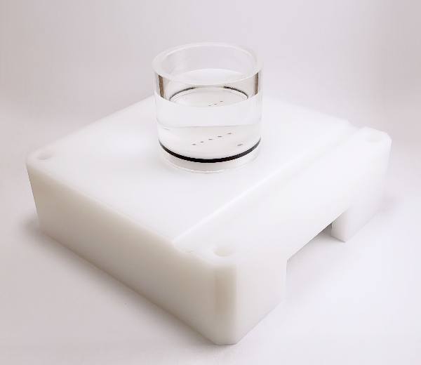
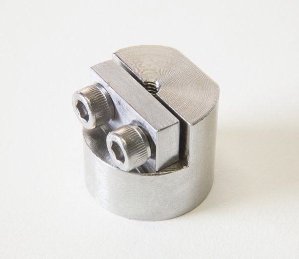
Round plate with screw clearances. Threaded to fit on MA626 test chamber

SKU: MA610 Categories: ,

This sample holder has been designed to secure in place an entire articular surface during 3D mechanical or thickness mapping protocol. A flat surface is created through the body of the bone underneath the articular surface to be tested. The flat bony surface is secured in place on the plate using wood screws passing through clearance holes from the bottom side of the plate. Screw length must be selected to ensure firm attachment of the sample while taking care of leaving the end of the screws far under the cartilage layer.

  • This accessory has been designed to facilitate cleaning and desinfection.
  • This part has a robust design and will keep its integrity for years
  • Designed to be used in contact with physiological saline solution
  • A knurling facilitates assembly
Material

Stainless Steel 316L

Diameter

86 mm, 5 mm (Hole)

Thickness

18 mm

Documents and resources (1)

Test configurations (4)

FAQ

What is the procedure to create a blank “.map” file?
NOTE. If no testing chamber is used proceed to step 5.

1. Completely screw the sample holder into the testing chamber and place the sample over it. If applicable, center the sample relative to the holder and rotate it in such a way that its orientation will approximately correspond to that of the corresponding surface positioning template image when seen by the technician in front of the testing chamber. Using a black marker, draw a mark on the top of the sample holder that will be used for the repositioning of the sample over the holder.

2. Remove the sample and unscrew the sample holder.

3. Depending on the sample type, a sample has to be attached to the sample holder following an appropriate method, either with screws and/or cyanoacrylate glue (recommended: Loctite 4013).

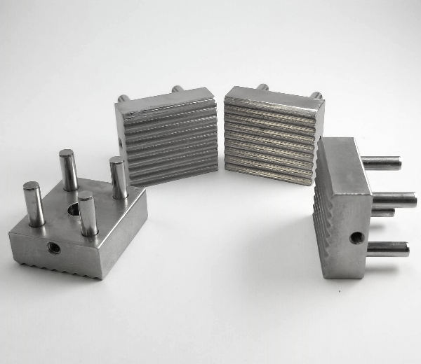
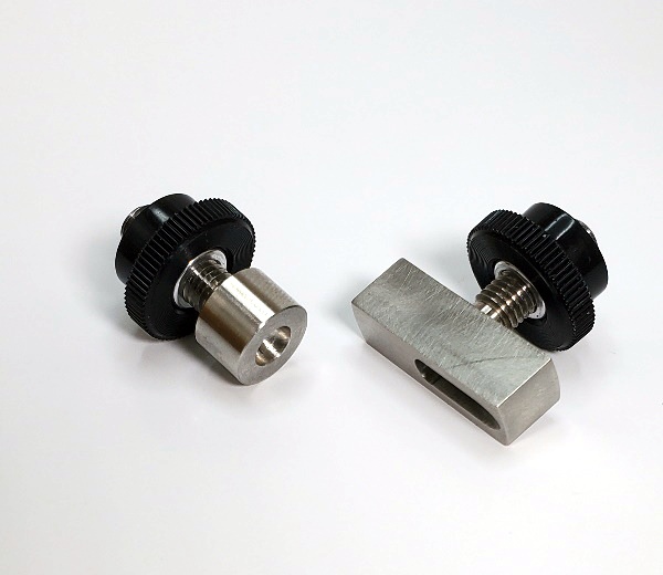
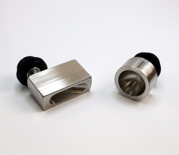
“Screws” method: In the case of sample holder (a – see Figure 1a), place the flat sample side in firm contact with the sample holder. Secure it with at least 2 screws from the bottom side. Make sure that the screws remain at least 1 cm away from the surface. In the case of sample holder (b – see Figure 1b), place the flat sample side in firm contact with the sample holder. Secure it from the periphery using its 6cone-ended screws. In the case of sample holder (c – see Figure 1c), place the sample in the middle. Secure it with its 2 screws.

“Glue” method: In the case of any sample holder with a flat portion (see Figure 1), make sure that the bottom surface of the sample and the flat portion of the sample holder are dry to ensure a good adherence. In the case of articular surfaces, apply the glue on the sample bottom (the bony part) and be careful not to touch the cartilage surface. If by mistake the glue touches the sample, try to clean the surface by using a flux of PBS, and report approximately the touched area in the laboratory book. The glued sample should be maintained for at least 1 minute to ensure a good adherence.

4. Screw the assembly into the testing chamber.

5. If required, create two reference points on the surface as per the “Calibration of the sample” section. If required, measure the horizontal distance between the references with a calibrated caliper and report the value (ideally, at a location specified in an associated protocol).

6. Adjust the position of the camera and its focus in such a way that the sample’s surface occupies the maximum space in the live camera feed while remaining completely visible by keeping a margin of about 5% at the 4 sides (right, left, up and down) to accommodate an eventual water refraction compensation, if applicable. It is recommended to use an appropriate surface positioning template to facilitate eventual mapping comparison between samples.
6.1. Choose “Import .map” in “File” of the menu bar.
6.2. Select the corresponding surface positioning template (*.map) and boundaries will be displayed by a closed contour (solid line) in the camera feed.
6.3. Adjust the position of the camera and its focus in such a way that the sample’s surface boundaries fit those of the surface positioning template.

7. Superimpose a position grid to the sample image. Positions could be added one by one according to a snapping grid (aligned) or anywhere on the sample. Also, positions could be imported through a previously created .map file. Note that it is important to edit/select a sub-surface in the Sub-SurfaceID field before adding a position in order to assign the position to a sub-surface.
7.1 If applicable, choose “Import .map” in “File” of the menu bar and select the corresponding position grid and the positions will be displayed by a circled marker in the camera feed.
7.2 If applicable, choose “Grid” in “View” of the menu bar to display a grid of snapping dots in the camera feed.
7.3 Edit the Sub-Surface ID field as defined in the associated protocol.
7.4 Choose “Add Positions” in “Edit” of the menu bar and click in the camera feed to add positions at each location of interest on the sample sub-surface.
7.5 If necessary, choose “Delete Positions” in “Edit” of the menu bar and click in the camera feed at each position that is not overlaid on a location of interest on the sample sub-surface and the position will be deleted from the camera feed.
7.6 Repeat steps 7.3 to 7.5 for each sub-surface of the sample.

8. If required, create the specific boundary of the sample sub-surfaces in order to refine the outline of the mapping surface for this specific sample (using at least 30 boundary points). If needed, surface boundary layer from the positioning template can be deleted first. Note that this step is important for the interpolation of characterization values to the boundary to obtain a complete mapping of the sample surface. Note that it is important to edit/select a sub-surface in the Sub-SurfaceID field before adding a boundary in order to assign the boundary to a sub-surface.
8.1. Choose “Boundary” in “View” of the menu bar to see boundaries in the camera feed.
8.2. Edit the Sub-Surface ID field as defined in the associated protocol.
8.3. Choose “Add Boundary” in “Edit” of the menu bar and click in the camera feed to define the boundary along the sample sub-surface and a closed contour will be created.
8.4. If necessary, choose “Delete Boundary” in “Edit” of the menu bar and click in the camera feed at a boundary point along the sample sub-surface and the closed contour will be reshaped consequently.
8.5. Repeat steps 8.2 to 8.4 for each sub-surface of the sample.

9. If required, add reference indicators on the two reference marks previously created at step 5.
9.1. Choose “Reference 1 (red)” in “Edit” of the menu bar and click in the camera feed at the first reference mark.
9.2. Choose “Reference 2 (blue) in “Edit” of the menu bar and click in the camera feed at the second reference mark.

10. Create this blank “Filename.map” file, where “Filename” is standardized filename format that it is recommended to define in an associated protocol (refer to Appendix I for a recommended file naming convention). When filename standardization is not necessary, any name can be used as “Filename”. Choose “Create .map” in “File” of the menu bar and all positions, boundaries and references displayed in the camera feed will be saved in the .map file and a snapshot image “.jpg” of the camera feed will be saved in the same folder.

Mapping Toolbox – Sample Holders

How does the "Interfaces Detection with Needle Probe" feature work?

This tool allows for the computing and visualizing of the surface position (mm) and the interface position (mm) of a “Find Contact” curve (load or force vs. position) obtained from a needle probe measurement (Jurvelin et al., 1995) on a sample (Figure 1). This model is well adapted for the thickness measurement of samples composed of two layers (a soft layer on top and a stiffer layer under), for example: articular surfaces. This analysis can be used in two modes, either automatic or manual. In the automatic mode, the low-pass filter cutoff frequency and the loading limit need to be specified in order to optimize the interface detection for each different sample. A user license is required in order to obtain the results of the interfaces detection with needle probe (Software Add-On, contact Biomomentum to obtain your license).

The needle probe measurement consists of moving the needle probe at a constant speed until it penetrates the surface of the sample and stops inside the interface. The difference between the position of the surface (position where the load starts to increase) and the position of the interface (sharp increase in the load) corresponds to the vertical thickness (Figure 2).

This analysis can be done in two modes, either automatic or manual. The automatic mode allows finding the surface (1) and the interface (2) position through an algorithm.

  • In order to find the surface position (1), the algorithm will start from the maximum load and will slowly scan the curve until the load will be equal to the load at the starting point (Figure 3).
  • In order to find the interface position (2), the algorithm will first smooth the curve with a low-pass filter (red line) and will then compute the first derivative (green line) and second derivative (blue line) of the curve. The position of the maxima of the second derivative will be considered as the interface position if its position is located before the user-defined loading limit (Figure 4).

Thus, the automatic mode consists of specifying two parameters:

Low-Pass Filter Cutoff Frequency (Hz) – Defines the cutoff frequency of the low-pass filter that will smooth the curve

Loading Limit (load/sec) – The inflection position is located before this loading limit defined by the user. This loading limit varies depending on the sample used; it represents the loading limit at which the user is certain that the needle probe is in the interface.

The manual mode lets the user drag the cursors to the surface the interface positions.
For example, (Figure 5) shows parameters used for the “Find Contact” function in needle probe measurement testing protocol on ovine articular surfaces. Corresponding results are shown in (Figure 1).

Mach-1 Analysis – Interfaces Detection with Needle Probe – Parameters

Mach-1 Analysis – Interfaces Detection with Needle Probe – Needle measurement

Mach-1 Analysis – Interfaces Detection with Needle Probe – Interface Position

Mach-1 Analysis – Interfaces Detection with Needle Probe – Surface Position

Mach-1 Analysis – Interfaces Detection with Needle Probe – Example

How does the "Elastic Model in Indentation" works?

This tool allows for the computing and visualizing of the shear modulus (MPa) and the Young’s modulus (MPa) from an indentation test performed using a spherical indenter (Figure 1). This model is well adapted for the mechanical characterization of samples (with critical diameter (width) at least 5 times the indenter diameter) bonded on a flat rigid support (at least 10 times stiffer than the sample), for example: any sheet of material lying on a rigid chamber base (limited sliding at the interface can be assumed) or a cartilage layer attached to a thick sub-chondral bone. A user license is required to obtain the results of the elastic model in indentation (Software Add-On, contact Biomomentum to obtain your license).

Results analysis is performed considering the indentation mechanics of an infinitely wide elastic layer bonded to a rigid half-space which has been developed as a model for the layered geometry of cartilage and subchondral bone (Hayes et al., 1972). (Figure 2) shows a schematic representing the modeled situation.

Many parameters need to be specified in order to calculate the different material properties.

1. Indenter Shape is:

  • Spherical
  • Plane-Ended Cylindrical

2. Indenter radius in mm.

3. Poisson ratio can be selected from a drop-down list (Figure 3)


4. Position @ contact is – defines the position of the left cursor:

  • to be curvefit – will automatically find the position contact which will give the smallest mean squared error (mse)
  • the value at t0 – will automatically take the position contact at the start of the curve
  • the following value (mm) – the user need to specify the value in the corresponding field next to the drop-down list
  • cursor position – the user can drag the left cursor to the wanted position contact

5. Sample thickness is the:

  • position @ contact – will automatically find the position at contact (position of the left cursor)
  • following value (mm) – the user need to specify the value in the corresponding field next to the drop-down list

6. Curvefit is up to – defines the position of the right cursor:

  • peak load – will automatically take the position of the peak load
  • delta load (unit) – the user need to specify the value of the desired delta load in the corresponding field next to the drop-down list
  • delta position (mm) – the user need to specify the value of the desired delta position in the corresponding field next to the drop-down list

The error on the estimation of the best curve representing the stress relaxation curve is calculated using the root of the mean squares (RMS) method and is displayed under “RMSE”. For example, (Figure 4) shows parameters used for the “Normal Indentation” (Mach-1 Motion) function in an indentation testing protocol on ovine articular surfaces. Corresponding results are shown in (Figure 1).

Spherical Indentation Guide – Mach-1 Mechanical Tester – Biomomentum

Mach-1 Analysis – Elastic Model in Indentation – Parameters

Mach-1 Analysis – Elastic Model in Indentation – Poisson ratio choices

Mach-1 Analysis – Elastic Model in Indentation – Cartilage & Subchondral bone

Mach-1 Analysis – Elastic Model in Indentation – Example

Need Help Choosing an Accessory?

Talk to our team

Report a problem with this page

Your email is used only to follow up on this report.

Screenshots (optional)

Click this area and paste a screenshot, or drag files here. Up to 3 PNG, JPEG or WebP images; 5 MB per image. Hide confidential information first.

Please do not include passwords or customer information. Reports and screenshots are private.